Face or no face (finding faces in photos using C# and Accord.NET)
I've always been intrigued as to how facial detection and recognition is handled by computers. It's one of the few effects that is seen in Hollywood films that seems convincing - where someone is tracked through a city, live CCTV feeds finding their face as they move from one street to the next. For a more mundane example, facial detection has been built into digital cameras and smartphones for quite some time now (my phone puts green squares around faces in photos and, I presume, uses this information to decide where to focus).
I knew literally nothing about the subject to begin with and so I hit the internet and tried to find out everything I could about it. Turns out that there's a lot that's been written about this, with various different methods and approaches discussed and documented. It's an interesting subject because it's been so affected by the rate of change in technology - for example, the digital cameras that introduced it had access to much less processing power than modern day devices do. I've had a hard time finding definitive information about when digital cameras started offering this facility but I'm getting a rough impression that it's over the last ten years (citation needed!) - when you think about how phones, for example, have changed in ten years in terms of their power.. well, it's a lot!
Having said that, digital cameras (and web cams) can take some shortcuts and only concern themselves with subjects that are facing directly towards the camera, since these are more likely to be subjects that are of interest - it's not as important to worry about people looking at ninety degrees from the camera lens, for example). So, straight away, it's apparent there are going to different techniques and different requirements for different situations and some will be more expensive than others.
I suspect that this is going to be an ongoing investigation for me; so far I've only managed to implement facial detection functionality and not facial recognition (once a face has been detected, is it someone from a database of known faces?). I thought I'd present what I have at this point, though - if it's interesting to me then maybe it will be of interest to other people! And I couldn't find much material out there that goes into enough detail that it's reproducible without being a really dense research paper (and certainly not ones that make it easy to reproduce their findings using C#), so I thought that I'd try to fill that gap. There are articles out there about using libraries to do all the hard work for you - but where's the fun in that?! I want to know how the code I'm calling is working.
tl;dr
My current code (github.com/ProductiveRage/FacialRecognition) identifies faces in photos by using two passes. First, it looks for regions of skin that have holes (that we presume may be eyes and a nose) and that are very roughly the right proportions to be a face.
The image content from these regions is passed through a "linear support vector machine", which will have been trained to classify a potential image region as a face or as not-a-face.
Before embarking on this adventure, I had no idea what a "support vector machine" even was. If you don't either then maybe you'll come away from this feeling like you know a little something about machine learning. I know that I did! And "machine learning" is a phrase that I've been interested in finding out more about for quite some time now, it seems like it's cropping up everywhere! I have a strong feeling that trying to perform facial recognition is going to involve even more magical sounding terms - such as "deep convolutional neural network" - but that's going to have to wait for another day, it's one (baby) step at a time for me.
The "Naked People Skin Filter"
In a past life, I worked in IT Support and, one day, I was asked by the Head Clinician why I'd been printing out porn. Which confused me considerably since I had most certainly not been printing out explicit material. There had been complaints about the colour tone and contrast of a new colour laser printer and so I'd sent a full-page test image to it that included greyscale content, colour grids and images that contained a lot of skin. Apparently printing out pictures with lots of skin in it raises eyebrows and maybe it's for similar reasons that a research paper entitled "Naked People Skin Filter" amusingly sounds a touch pervy (or maybe that's just a British thing.. we do love to keep most of our naked-skin-unveiling behind closed doors - because it's so cold!).
This "Naked People Skin Filter" paper was published by Margaret M. Fleck and David A Forsyth and is available at http://mfleck.cs.illinois.edu/naked-skin.html. It essentially describes an algorithm to detect regions of skin in an image. In 1997, another paper "Face Detection in Color Images" described starting with that skin-tone-identifying approach and then using it to try to find solid regions of skin that have a few holes in, on the basis that this is probably a face (where the holes are eyes, nose, mouth).
Note: That "Face Detection in Color Images" link use the Wayback Machine to make available a GeoCities page. Maybe it's a sad reminder that there was actually worthwhile content on GeoCities as well as the many harshly-coloured-and-bizarrely-animated eye-watering monstrosities. By the way, if you (quite rightly, imho) think that the web has lost something by having less places for people to upload content for free then check out NeoCities - it's awesome because it makes that possible again (and all the good and bad that comes with it)!
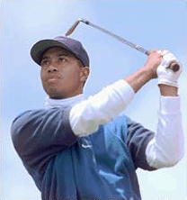
"Face Detection in Color Images" uses an example image of Tiger Woods and so I will use that same image while I discuss what I've done, based upon these articles.
There are a set of steps that are followed when trying to identify faces in an image:
- Scale the image down (depending upon its size)
- Avoid desaturation by bring colour down values so that the minimum is true zero
- Transform RGB colours into the RG/BY colour space, alongside an Intensity spectrum
- Calculate "texture amplitude" across the image (how quickly intensity changes - the theory is that areas of skin have a relatively low texture amplitude)
- Calculate hue and saturation across the image (in order to identify areas that seem to be skin-coloured)
- Combine the texture amplitude and hue data to identify areas of skin (the texture amplitude, hue and saturation must be within acceptable "this is probably skin" bounds)
- Expand these areas of skin using a more relaxed texture amplitude / hue / saturation "this is probably skin" filter
- Check these areas for holes - no holes (for non-skin facial features, such as eyes) means no face
- Any skin areas that are very small are ignored
- Any skin areas that are extreme aspect ratios are ignored (very, very wide areas or very, very tall areas are probably not faces)
- Expand the areas slightly because, even with the flexible-skin-filter expansions, the area that a human would identify as being a person's face is slightly larger than the areas identified by this algorithm
Calculating hue, saturation and texture amplitude (steps 1-7) to identify skin areas
The first few steps are fairly simple. If the image is either taller or wider than 400px then it's shrunk down so that the largest side is 400px. "Naked People Skin Filter" talks about applying "smoothing" (which I'll cover in a moment) relative to the size of the image but doesn't suggest any restrictions on the image size. "Face Detection in Color Images" mentions that only images up to 250px were used. With the test images I used, I found that capping at 400px provided a reasonable balance between identifying faces and not taking too long to process. I used the Tiger Woods image initially to try to ensure that my calculations were matching those described in "Face Detection in Color Images" but I used other test images (which will appear further down) to double-check that everything seemed to be working as expected. There are some differences between how Fleck & Forsyth ("Naked People Skin Filter") and Kapur ("Face Detection in Colour Images") perform the analysis and my test images led me to tweak a few parameters myself.
Fleck & Forsyth recommend pulling down the colour values so that the minimum value is zero because it "avoids potentially significant desaturation of opponent color values if the zero-response is far from zero". What this means is that the darkest parts of an image are probably not "true black" (ie. RGB 0, 0, 0) and the theory is that we should get better results if everything is adjusted down so that the darkest colour is black. In practice, I look for the lowest of any of the R, G or B values from any pixel in the image and subtract that value from every R, G and B value across all pixels in the image.
Next, I generate "RgByI" values for every pixel. This a trio of values; an RG (red-green) spectrum value, a BY (blue-yellow) spectrum value and an intensity. Since I'm going to spend a lot of time taking the pixels from an image and loading them into a 2D array and then performing a range of operations on them, I've written a DataRectangle<T> class that makes this easier. When I first read the data from an image, the pixels are loaded and used to populate a DataRectangle of RGB values. When I need to get RgByI values from them, I can do the following (using Kapur's formulae from "Face Detection in Colour Images) -
var rgByIValues = colourData.Transform(colour =>
{
    Func<byte, double> L = x => (105 * Math.Log10(x + 1));
    return new IRgBy(
        rg: L(colour.R) - L(colour.G),
        by: L(colour.B) - ((L(colour.G) + L(colour.R)) / 2),
        i: (L(colour.R) + L(colour.B) + L(colour.G)) / 3
    );
});
In order to reduce unhelpful detail in the image somewhat, the RgByI values have a "windowing median filter" applied to them. From "Face Detection in Colour Images" -
The Rg and By matrices are then filtered with a windowing median filter .. with sides of length 4*SCALE. The SCALE value is calculated as being the closest integer value to (height+width)/320
(The "Naked People Skin Filter" paper recommends using 2*SCALE for the RG and BY values, which I have gone with because I found the results to be just as accurate and it's less computational work than 4*SCALE)
To do this, you go through every pixel and take its value and the values from the surrounding pixels, sort them, take the middle value (the "median") and use that as the new value for the current pixel. The idea is that this reduces noise by discarding any outlier pixel colours in a given range. I take a square block around where the initial pixel is but it would probably be better to approximate a circular area if the media filter radius is large (in my filter, it's never more than three).
After smoothing the RG/BY data, their values are combined to generate hue and saturation -
var smoothedHues = smoothedRG.CombineWith(
    smoothedBY,
    (rg, by) => new
    {
        Hue = RadianToDegree(Math.Atan2(rg, by)),
        Saturation = Math.Sqrt((rg * rg) + (by * by))
    }
);
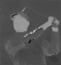
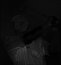
The two images here are the hue and saturation values generated from the original image.
In order to generate greyscale images, I had to translate the hue and saturation values into the 0-255 range. The hue values will be in the range of -180 to +180 degrees so I just added 180 and then divided by 2. The saturation values are always positive and won't exceed 0-255 if multiplied by 2, so I just did that.
Generating texture amplitude is more complicated. We start with the intensity values from the RgByI data. We then run that through a median filter of 2 * SCALE and calculate the difference between every point in the median filter result and the original intensity. Finally, we run the result of the calculation through a median filter of 3 * SCALE. It may be clearer with some code -
var smoothedIntensity = rgByIValues.MedianFilter(
    value => value.I,
    2 * scale
);
var differenceBetweenOriginalIntensityAndSmoothedIntensity = rgByIValues.CombineWith(
    smoothedIntensity,
    (x, y) => Math.Abs(x.I - y)
);
var textureAmplitude = differenceBetweenOriginalIntensityAndSmoothedIntensity.MedianFilter(
    value => value,
    3 * scale
);
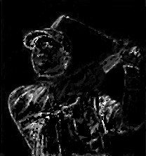
(Note that the values 2 and 3 in the above code are much lower than Kapur suggests - 8*SCALE and 12*SCALE - but the median filtering algorithm that I threw together was very slow using the higher values and using lower values - which meant that the processing completed much more quickly - did not seem to affect the outcomes)
Hopefully it's apparent that around the lower face there is low texture amplitude. Texture amplitude is higher around the facial features but that's to expected. There is low texture amplitude elsewhere in the image (particularly in the sky behind him, the texture is very smooth there and so the texture amplitude is very low) but what we're going to look for is areas that appear to be skin in hue/saturation and in texture amplitude.
Now that we have all of the information required to guess whether a given pixel is within the acceptable bounds of "probably skin", we can create a skin mask (a DataRectangle<bool>) -
var skinMask = smoothedHues
    .CombineWith(textureAmplitude, (hs, t) => new
    {
        Hue = hs.Hue,
        Saturation = hs.Saturation,
        TextureAmplitude = t
    })
    .Transform(hst =>
    {
        return (
            ((hst.Hue >= 105) && (hst.Hue <= 160) && (hst.Saturation >= 10) && (hst.Saturation <= 60)) ||
            ((hst.Hue >= 160) && (hst.Hue <= 180) && (hst.Saturation >= 30) && (hst.Saturation <= 30))
        )
        && (hst.TextureAmplitude <= 5);
    });
This is another point at which I have added my own tweaks to the processing. There are slightly different ranges of acceptable hue / saturation / texture amplitude suggested by Fleck & Forsyth than are suggested by Kaypur and I found that I wanted to change them a little based upon the test images that I was using.
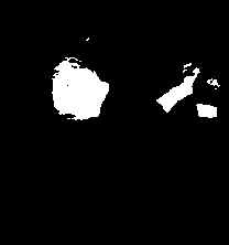
The final step in generating the skin mask is to try to identify any skin areas just outside the identified mask. I've used the approach suggested by Kapur, who recommends it because it "helps to enlarge the skin map regions to include skin/background border pixels, regions near hair or other features, or desaturated areas".
The idea is that we look at negative values in the DataRectangle<bool> skin mask and check whether any of the adjacent values is positive and if the colour of the pixels that resulted in the false value passes a more relaxed skin filter. The relaxed skin filter test demands only that the hue is within the range 110-180 and that the saturation is with 0-180 (the text amplitude is not considered). This expansion work is performed twice.
Recognising skin objects (and checking for holes)
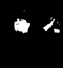
In order to get back some of the details that are within the skin mask areas, the original image is changed to greyscale and then the skin mask is combined with it to produce a new skin mask that is slightly more restrictive; any negative content from the skin mask remains negative while positive content is only allowed if the greyscale intensity is within an acceptable range. Everything from this point (including this step) comes from the "Face Detection in Color Images" article, since "Naked People Skin Filter" ends when the skin regions are detected (it has no interest in faces, specifically).
skinMask = colourData.CombineWith(
    skinMask,
    (colour, mask) =>
    {
        if (!mask)
            return false;
        var intensity = colour.ToGreyScale();
        return (intensity >= 90) && (intensity <= 240);
    }
);
In order to turn this DataRectangle<bool> mask into groups of points (where each group represents a distinct area of skin), I used a variation of the "Stack based implementation" from this article: Flood Fill algorithm (using C#.Net). If you're looking my code, it's the "TryToGetPointsInObject" method in the FaceDetector.cs class. I'm not stressing out about performance at this point, I just wanted to get things working and then considering measuring & improving in the future - so finding a nice simple flood fill algorithm was very helpful (I'm not saying that it's not a well-performing method, I'm just saying that at this point in time it's not critically important to me one way or the other).
Any skin objects that are very small (have less than 64 * SCALE points) are ignored. What is slightly more complicated is to identify any completely enclosed holes in the skin object. But it's not much more complicated - the basic approach is, for each skin object, take a negative point within the bounds of the skin object and use the flood fill algorithm again; if the fill reaches the edges of the bounds then the negative point was not part of an enclosed hole. Then move on to the next negative point within the bounds that hasn't already been included in a flood fill operation and continue doing this until a fully enclosed hole is found that's larger than a given size (1 * SCALE).
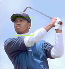
With the Tiger Woods image, we could actually stop here. It successfully identifies only his face as a possible face region. However, with other test images I used, some more work was required. I found that I could quite easily eliminate a few false positives by ignoring any regions that were obviously the wrong aspect ratio (either very long and shallow sections or very tall and narrow sections). I also found that, depending upon lighting or what background a face was against, sometimes the detection process up to this point would result in a region that is too tight over the facial features - expanding the matched area a little meant that the next filtering in the next stage would get better results.
The real problem, though, is false positives - the algorithm will often identify areas that are not faces.
Applying this to other images
I wanted to try applying this facial detection logic to some other images. I'd used the image from one of the articles so that I could try to produce intermediate images that looked similar to those in "Face Detection in Color Images" so that I could reassure myself that I was (at least approximately) doing things correctly as described. But now I wanted to try it on some other test images.
In my Pictures folder, some photos from an Easter weekend* night out I went to a couple of years ago jumped out at me. Initially, I only used them because they made me laugh but, on closer inspection, they're actually really useful for illustrating what the skin tone detection process (and the subsequent support vector machine classification) is good at and where their limitations come into play.
* (which goes some way to explaining the eggs and the costumes.. the photos were put up on Facebook by a professional photographer, I hope he doesn't mind me reproducing them here - I tried getting in touch to ask but he didn't get back to me)
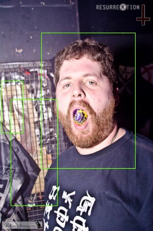
Firstly, we have this fine gentleman. The skin tone pass has identified his face perfectly but it's also misidentified two regions that contain colours and textures that the skin filter allows through.
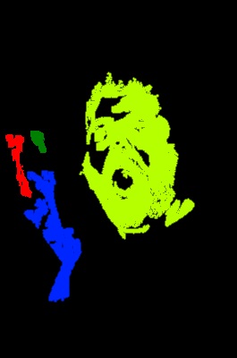
Looking at the generated skin mask (where each distinct skin object is filled with a different colour), it should be clear why this has happened.
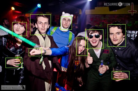
If we take another photo then another problem is apparent - with this group of people, there are lots of enclosed skin objects that have holes in that are being identified as faces but that are actually hands holding things.
Also, because we ignore regions that are very small, there is a limit to what faces the skin tone filter will identify. If you look closely at the group photo there is an undetected bearded face along the left edge (near the top) but I am happy for it to exclude him since I think that it is a reasonable compromise to prefer faces that are in the foreground. On the whole, it does a good job of detecting faces but it may also produce a lot of false positives.
So the next step is to try to find a way to filter these regions down further, to try to get rid of those pesky false positives. To do this, I went back to the internet. One of the pages that I found incredibly useful was the "HOG Person Detector Tutorial" by Chris McCormick. He introduces a popular and modern technique, touches on its history and then goes into an illustrated explanation of how to implement it. It's almost redundant me going over it again! .. but it's my blog and I'm talking about how I implemented it, so I'm going to start from the beginning anyway :)
At the very highest level, what we're going to do is this -
- Take a load of images that are known to be faces and a load of images that are known to not be faces - these sets of "positive" and "negative" images are our "training data"
- Extract a load of numbers from each image - each image must be processed in a manner that results in them each producing the same amount of numbers (this is called "feature extraction")
- The resulting data (which is a big list of entries, one from each training image, where each entry is a list of features from that image and a boolean value for whether the image was a face or not) is used to train a "Support Vector Machine" (which I'll explain in a second)
- Now that we have a trained SVM, we can use the same feature extraction process from step 2 on each of the sub-images generated by the skin tone detection process and the SVM should tell us whether each one is a face or not a face
So what is a Support Vector Machine?
This is a concept that I had never heard of before, so I know first-hand what it's like trying to search around on the internet for a good description. The problem is that a lot of articles seem to be aimed at people who know at least something about machine learning and they go immediately to showing lots of formulae and talking about techniques that I'd never heard of. One example is "Kernel Support Vector Machines for Classification and Regression in C#" by César Souza (who wrote much, if not all, of the Accord.NET library - which I will be using later); this is a really well-written article that I appreciate now but it was on my "come back to this when you know more" list for quite a while after I first found it!
So I'm going to take a real beginner approach and try to describe it in a manner that would have helped me a few weeks ago.
Firstly, an SVM tends to be a "binary classifier". This means that it will be trained with data that is all categorised as either yes or no. After it has been trained, you may only ask it to classify further data as being a yes-or-no result. (Actually, there is a such a thing as a "Multi-Class Support Vector Machine" that can return a greater range than binary but it's not relevant here so I'm going to forget about it for now).
(Time for some graphs. Shout out to Create your own XKCD-style Graphs, which helped me come up with what's below!)
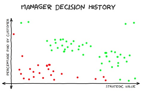
To conjure up an example that almost sounds feasible, imagine that every development task at a software shop requires that its strategic benefit to the company be quantified, along with the percentage of the work that a customer is just dying to pay in order for it to be done (presuming that there is a customer who wants it and that it's not just a task for internal purposes). Since every task needs to have these pieces of information before your manager will decide whether or not the work will be scheduled, there exists historical records of estimated tasks which have two "features" (strategic value and percentage-that-will-be-immediately-paid-for-by-customers) and an outcome of either "yes, it was done" or "no, we didn't do it".
If something is of high strategic value to us and it happens to be a feature that a customer is chomping at the bit for (and so will contribute significantly towards) then it seems like a dead cert that we should do it. Unfortunately, this is not a very common case.. More often, a customer will want something that is important to them specifically. This may not be something that is necessarily very easy to resell to other customers (which would give it more strategic value) or something that will help us deal with internal issues, such as scaleability or technical debt (developments that do help with those will also have higher strategic value).
It seems like there's a roughly linear correlation between a development's strategic value, the fraction that customer(s) are willing to immediately pay for it and whether the work got the go-ahead. It's like we could draw a line and everything above it tends to get the green light by our manager and everything below it gets rejected.
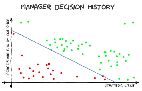
An SVM is (according to wikipedia), a:
"model with associated learning algorithms.. An SVM model is a representation of the examples as points in space, mapped so that the examples of the separate categories are divided by a clear gap that is as wide as possible"
What this boils down to is that we're essentially trying to come up with a formula to split those two sets of points. Then, when we get a new feature-pair (strategic value vs amount-customer-will-pay) we can plug those two numbers into the formula and work out which side of the line we're on (where one side means I-predict-yes and the other side means I-predict-no).
The hard work in the machine learning algorithm is working out where that line should go. Ideally, you want all historical "yes" results on one side and all historical "no" results on the other side. In some cases, though, this is not possible and there will be some outliers (remember that task that you had to do that seemed to have no strategic value, that no customer was willing to pay for and yet someone at one of those customer companies had convinced one of your directors to do it at as a favour...?). Whether there are any outliers or not, there are probably still many slight variations on what line could be drawn. It's common for an algorithm to try to arrange the line so that it is equally distant from the positive results as it is from the negative results but there are some variations on this theme. This is really what the magic is in this process - giving the computer the results and letting it find the best match.
Higher dimension planes and non-linear methods
In the above example, each data point only had two features which made it very easy to envisage on a 2D graph how they related to each other (which isn't surprising since it's an example I made up to illustrate that very point!). Sometimes, though, more data is required. It could be that you plotted strategic-value against amount-customer-will-pay and could see no correlation, though one was there - but hidden due to the interaction of another feature. Imagine if you find historical data that shows that a customer wanted to pay for a new feature and the feature was of reasonable strategic value but it wasn't authorised. Or if there were a bunch features with comparatively low value that did get the go-ahead. And if you realised that these were not outliers and that lots of results looked to be "all over the place". Well, it could be that the reason that the high value work wasn't done was because the development team were already stacked out with important work. Whereas those low value jobs that did get done happened to come in during quiet periods where they could be easily slotted into the schedule. This would mean that there was actually a third factor at play; available developer resources.
What would be required to model this would be to include some quantified "available developer resources" value with each data point. With this additional information, we should be able to construct a useful prediction model. However, the points could no longer be plotted on a simple 2D graph - now they would have to be plotted in 3D space. And so the formula that would be produced from the training data would no longer draw a simple line, it would have to describe a plane that cuts through the 3D space (with the "yes" values on one side and the "no" values on the other).
If you had more than three features to each data point then you would no longer be able to draw a graph of it, your points would now live in the mysterious-sounding "n-dimensional space". It's still possible to concoct a formula that divides the data point within that space, it's just not very easy to imagine it in a visual manner. On the 2D graph, it was a one-dimensional line that split the data points and allowed us to make predictions against future data points. On the 3D graph, it would be a two-dimensional plane that divides the points. In n-dimensional space, it will be a "hyperplane" (which just means that it is a structure with one less dimension than the space that it exists in). Once you start throwing terms around like "Linear SVM" and "hyperplane", it's hard not to feel like you're making real progress towards getting a handle on all this machine learning lark! I mention these higher dimensional spaces, though, not just because they sound exciting but because they will be relevant soon..
Something else that's interesting when considering SVMs is that, even with all of the required data, it still might not be possible to delineate the positive and negative results with a linear formula. If we go back to imagining a 2D graph, there could be curious curves in the data that are predictable but can not be cleanly cut with a straight line. In this case, we would have two choices - have the algorithm try to find a line that cuts the results as well as possible (but accept that this will have a lower accuracy because we know that a straight line will get a lot of predictions wrong, based upon the data we've got) or we can allow it to try to come up with a non-linear separation.
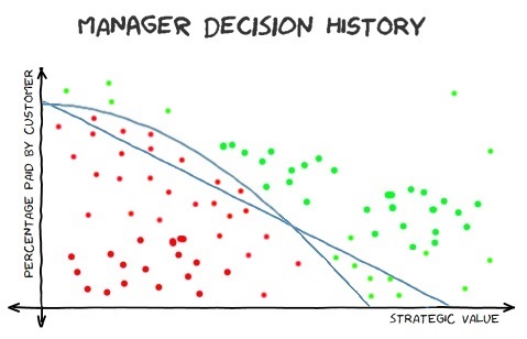
If, say, you had a manager who leant more towards authorising tasks that had greater strategic value, even if there weren't immediately customers to finance the work (maybe they favour tasks that improve efficiency for work that customers are excited about or maybe it's to lay the groundwork required before customer-led work can continue) then it might not be possible to perfectly fit a straight line to the data. One option, when trying to model this, would be to specify that the learning algorithm could use a non-linear kernel, would would hopefully generate better predictions. Or you could stick with the linear approach and accept that it will be less accurate. Looking at the graph here, there is a curved line that matches the data precisely and there is a straight line that tries its best but can't help splitting the data so that some negative values are above the line (where only positive values should be) and some positive values are below the line (where only negative values should be).
This is another illustration that machine learning can't perform miracles. Before, I described an example where a third feature would need to be added to the data ("available developer resources") - without which it would be impossible to train a useful model. Here, we can see that sometimes we need to have some insight into what prediction models may or may not work for us (ie. we need to know that a linear kernel won't yield the best results).
I'm not going to dwell on this any longer here because, happily, a linear SVM is a good fit for the data that we'll be working with for classifying face / not-a-face. I don't think that I yet understand enough about the subject to explain why a linear model works so well for what we want to do but I do have links to articles (which I'll include at the end of this post) that seem happy to explain why this is the case.
Feature extraction for maybe-a-face images
So, if an SVM can be trained on pre-existing data and then used to decide whether other data (that it's never seen before) should be classified as a yes or a no, how can this be applied to our "potential face regions"? The first thing that we need to do is decide how to extract features from an image. In the "Manager Decision History" examples above, there were only two or three features but there's nothing stopping us from extracting many more features from our inputs. Whatever we do, though, we need to generate the same number of features for every input into the SVM - so we'll almost certainly have to resize each maybe-a-face sub-image before processing it. We could consider taking all of the pixel data from each resized sub-image (every red value, green value and blue value from every pixel across the entire sub-image).. but we're not going to. Not only would there be a lot of data to work with, there would also be too much variance introduced by the environment of the source photograph. We want to try to give the SVM meaningful data for it to analyse and remove irrelevant variables where possible. By "irrelevant variables", I mean that it would be great if we could ignore the lighting in an image and focus on the shapes.
Sometimes the lighting varies not just from one image to another but within the same image - if there is a person outside and sunlight falls on one side of them, for example. And it would be great if we could ignore the contrast and the shades of colour - if you can imagine fiddling with an image in Photoshop (or the excellent Paint.NET), recolouring an image or playing with the contrast and brightness doesn't affect your ability to recognise what's in the image (unless you really stretch some of those dials to the max) and we don't want those sorts of differences to have any impact on the SVM's predictions. What we really want is to discount as much of this variance as possible when preparing the inputs (both the inputs used to train it and the subsequent inputs that we want predictions for).
A method that works well to achieve this is to generate normalised "Histograms of Oriented Gradients" from the sub-image. Again, I've come to this conclusion from doing a lot of reading around and then attempting to implement described methods to see how they work - I'll include references to articles with more details at the end of this post.
The premise is fairly simple, you need to:
- Ensure that every image to process is a consistent size before starting (if an image is the wrong aspect ratio for whatever the "consistent size" that you decide on is then add some black bars above-below or left-right, depending upon which sides are too long/short)
- Greyscale the image
- For every pixel, work out the direction that the intensity of light on the image is changing and how quickly it's changing
- Split the data into blocks
- Reduce each block into a histogram of gradients
- Apply some sort of normalisation to reduce impact of contrast or brightness differences from image to image
- Use the resulting data as the image's feature set in the next step!
I think that steps 3 and 5 are probably the ones that require further explanation. Since we have a greyscale image by step 3, instead of colour data we effectively have "intensity" values for each pixel. To work out the angle in which the intensity is changing, take the intensity of the pixel below the current one and substract it from the intensity of the pixel above the current one. This is the "y difference" - or "delta y", so I'll name it "dy" (so that I can sound all maths-y). "dx", as you can probably imagine, is the difference between the intensity of the pixel to the right minus the intensity of the pixel to the left. We can calculate the angle at which intensity is changing (and how big the change is) with the following:
var angleInDegrees = RadiansToDegrees(Math.Atan2(dx, dy)));
var magnitude = Math.Sqrt((dx * dx) + (dy * dy));
Note that "Math.Atan2" returns a value in radians. Radians are another unit of measurement of angles but instead of describing a full circle by going from 0-360 degrees, the scale goes from 0-2π radians. So, to convert from radians into easier-to-deal-with-in-this-case degrees we can do this:
private static double RadiansToDegrees(double angle)
{
    return angle * (180d / Math.PI);
}
Also note that Atan2 actually returns values in the range of -π to +π and so calling RadiansToDegrees on the result will give us a value from -180 to +180.
(When calculating gradient angles and magnitudes, any pixels on image edges won't have pixels surrounding in every direction and so I just record them as having both an angle and magnitude of zero)
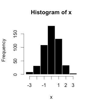
Now for step 5, we want to produce "histograms of oriented gradients" (one for each block that we've split the image into in step 4). I always envisage a histogram like a bar chart - it shows how values are distributed across a range.
(The example on the left is from wikipedia and reproduced here under the creative commons license)
To generate our histograms, we want to assign the gradients with the block across nine buckets, spaced twenty-degrees apart. The first will be at 10 degrees, the second at 30 and they'll go all the way up to 170.
We're going to use "unsigned gradients", which means that if we have a gradient where intensity is changing only vertically, we don't really care if it's getting brighter as it goes down or brighter as it goes up, we only care that the line is precisely vertical. Similarly, imagine the intensity increasing up-and-right, at 45 degrees - we're happy to treat this the same as intensity going in precisely the opposite direction; down-and-left and 225 degrees (or -135 degrees since our current angleInDegrees values are in the -180 to +180 range). What this essentially means is that we want to tweak our angles so that they are all within 0-180 (instead of -180 to +180). To do, so we just add 180 degrees to any values less than zero.
Every gradient needs to be assigned to one or more of these buckets. If a gradient's angle is precisely 10 degrees then the entirety of the gradient's magnitude is added to the 10 bucket. However, if it's between 10 and 30 then its magnitude is split proportionally between 10 and 30 (so a gradient of 20 degrees is split evenly between 10 and 30 while a gradient of 25 degrees will contribute 3/4 of its magnitude to the 30 bucket - which it is 5 degrees away from - and 1/4 of its magnitude to the 10 bucket - which it is 15 degrees away from).
Performing this transformation on the image is an effective way of reducing the amount of data that we need to deal with. If we decide that the standardised size of the images that we want an SVM to classify is 128x128 then we 128 x 128 x 3 = 49,152 values (since every pixel has three colour values; red, green and blue). If use a block size of 8 when generating the HOG data then the 128 x 128 image will be 16 x 16 blocks and each block has 9 values (since each histogram has values in nine bins), which gives a total of 2,304 values.
Another nice thing about this representation of the data is that, if you sort of squint, you can kind of make out the shapes that were in the source image -
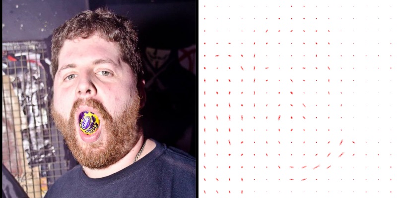
If you get curious and want to try generating HOGs for your own images, there is code in my my GitHub project to do this..
using (var image = new Bitmap(imagePath))
{
    using (var resizedImage = new Bitmap(image, new Size(128, 128)))
    {
        // (Can ignore GetFor's return value when only interested in generating a preview image)
        FaceClassifier.FeatureExtractor.GetFor(
            resizedImage,
            blockSize: 8,
            optionalHogPreviewImagePath: "HOG.png",
            normaliser: GlobalNormaliser.Normalise
        );
    }
}
.. which brings me neatly on to HOG normalisation (since there's a mysterious reference to a normaliser in the code above). When the gradient magnitudes are calculated, some images may have many pixels that vary wildly in intensity from their neighbours while other images may have smoother, gentler gradients. In both cases, it is the relative flow of intensity that is important, since that helps identify the shapes. If you took an image and produced HOG data for it and then increased the contrast of the image and re-processed it, you would get greater gradient magnitude values in the increased-contrast version of the image, even though they both - so far as we are interested (in the context of trying to detect faces) - contain exactly the same information.
What we want to do is to align all of the magnitudes to a common base line. A simple (and fairly effective) way to do this is to find the largest value of any of the buckets across all of the histograms generated for an image and to then divide every magnitude by this value. In the example above, the 128x128 input image is transformed into 16x16 blocks, each of which is a histogram that contains 9 values. So we get the largest value from each of those 16x16x9 values and then divide all of them by it. This means that the largest value is now precisely 1.0 and every other value is somewhere between zero and one. This is what the "GlobalNormaliser.Normalise" delegate in the code above does. All it essentially has to do is this:
public static DataRectangle<HistogramOfGradient> Normalise(DataRectangle<HistogramOfGradient> hogs)
{
    if (hogs == null)
        throw new ArgumentNullException(nameof(hogs));

    var maxMagnitude = hogs.Enumerate()
        .Select(pointAndHistogram => pointAndHistogram.Item2)
        .Max(histogram => histogram.GreatestMagnitude);
    return hogs.Transform(hog => hog.Multiply(1 / maxMagnitude));
}
However, there is a variation on this that has been found to produce more accurate results; "block normalisation". The original description of this process comes from (as I understand it) the original research into using HOGs for this form of detection ("Histograms of Oriented Gradients for Human Detection [PDF]") -
For better invariance to illumination, shadowing, etc., it is also useful to contrast-normalize the local
responses before using them. This can be done by accumulating a measure of local histogram “energy” over somewhat larger spatial regions (“blocks”) and using the results to normalize all of the cells in the block
What this means in practical terms is explained well by one of the articles that I linked earlier ("HOG Person Detector Tutorial"). In essence, it means that we can get better results from normalising over smaller areas of the image. Instead of taking the max magnitude across the entire set of data, the idea is to group the histograms into blocks of four and normalising over those.
Let's go back to Tiger Woods' face to illustrate what I mean.
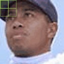
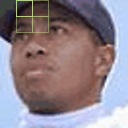
We first take the 2x2 histograms from the top left of the image - we get the max magnitude from within those four histograms and use it to normalise the values within them. These four normalised histograms will provide the first sets of values that we extract from the image.
Then we move across one to get another set of 2x2 histograms and repeat the process; get the max magnitude from within those four histograms, use it to normalise them and then take those four normalised histograms as the next set of values that we have extracted from the image.
What you might notice here is that, as we look at the 2x2 blocks of histograms, some of them will appear multiple times. The histograms from the edges of the image won't but the others will. In the Tiger images here, you can see that the two histograms at the right hand side of the block in the first image are included again in the second image (now they are the two histograms on the left hand side of the block).
This means that this "block normalisation" process will result in more data being produced. When we "globally normalised" the HOGs then we had 16x16x9 = 2,304 values. However, if we block-normalise (using blocks of 2x2) then we generate 30 blocks across (there are two edge blocks that are only counted once but the other 14 blocks are all counted twice, so the total is 2 + (14*2) = 30). For the same reason, we will generate 30 blocks worth of data as we go down the image. This means that we end up with a total of 30x30x9 = 8,100 values.
To extract those features, we would tweak the code from before -
const int inputWidth = 128;
const int inputHeight = 128;
const int blockSizeForHogGeneration = 8;
const int blockSizeForLocalNormalisation = 2;

IEnumerable<double> features;
using (var image = new Bitmap(imagePath))
{
    using (var resizedImage = new Bitmap(image, new Size(inputWidth, inputHeight)))
    {
        var blockNormaliser = new OverlappingBlockwiseNormaliser(blockSizeForLocalNormalisation);
        features = FaceClassifier.FeatureExtractor.GetFor(
            resizedImage,
            blockSize: blockSizeForHogGeneration,
            optionalHogPreviewImagePath: null,
            normaliser: blockNormaliser.Normalise
        );
    }
}
(Note that I'm setting "optionalHogPreviewImagePath" to null so that "FeatureExtractor.GetFor" doesn't generate a "HOG preview" image - this is because it's much harder to recognise the shapes that the gradients were extracted from when this form of normalisation is use since most of the HOGs appear multiple times, so the preview images are of less interest)
When I tried comparing the results of global normalisation vs block normalisation, I found that I got better result (ie. better accuracy) when using block normalisation, just as the authors of "Histograms of Oriented Gradients for Human Detection" did. The number of images that I've been testing with is, I'm sure, much smaller than the number used by Dalal and Triggs in their research but it was gratifying that I could see improvements with my data set from using block normalisation - if only because it reassured me that I was moving in the right direction!
Training an SVM
It's really coming together now. We've got a way to extract data from an image that we will be able to pass to an SVM in order for it to classify the image as "face" or "not face". There's just one thing that we're missing.. a trained SVM. Or, another way to look at it, two things we're missing - a mechanism to train an SVM and the data to train it with.
Let's start with a general way to train an SVM. For this, I'm going to use a package called Accord.NET. It's a library entirely written in C#, which was a plus to me because I like to see how things work and when I was doing my early reading around on the subject of face detection/recognition, a lot of people were recommending OpenCV. This is a C++ library (which can be called by C# using a .NET wrapper called Emgu), while I would be happier with C# source code that I could more confidently dig around in. (Also, I'm toying with the idea of trying to port some of this work to a Bridge.NET project so that I can try making it work in the browser - this wouldn't be possible if I took a dependency on a library like OpenCV).
Accord.NET really does make it easy.. once you know where to get started. There are a lot of examples on the accord-framework.net site and on the GitHub wiki, though some of the code samples are out of date and will generate compile warnings if you try to use them directly. (Having said that, the warnings can be ignored and it's not too hard to find other examples that compile without warnings - and, from reading some of the GitHub issues, I know that César is aware that some of the docs need updating and is intending to do so when he can make time).
To demonstrate, let's revisit the "Manager Decision History" example from earlier. We'll formulate some example data where we pretend that the Manager is super-consistent and will always authorise work if the percentage that the customer will pay for immediately (as a value between 0 and 1) plus the strategic value (also somehow quantified as a value from 0 to 1) add up to more than 1. (So strategic value 0.9 plus customer-will-pay-immediately 0.2 will be authorised as 0.9 + 0.2 > 1 but strategic value 0.8 with customer-will-pay-immediately of 0.15 will not be authorised as 0.8 + 0.15 < 1). We can then use that data to train an SVM and then try other values against the model -
// Make up some data (in the real world we'd use some proper pre-classified training
// data but this is just an example to demonstate how to train an SVM using Accord.NET)
var decisionHistory = Enumerable.Range(0, 10).Select(x => x / 10d)
    .SelectMany(x => Enumerable.Range(0, 10).Select(y => y / 10d).Select(y => new
    {
        StrategicValue = x,
        ImmediateCustomerContribution = y,
        Authorised = (x + y) > 1
    }));

// From the data, extract the input features (strategic-value and amount-customer-will-
// pay-now)..
var inputs = decisionHistory
    .Select(decision => new[]
    {
        decision.StrategicValue,
        decision.ImmediateCustomerContribution
    })
    .ToArrary();

// .. and the true/false outputs for each of those sets of features
var outputs = decisionHistory.Select(decision => decision.Authorised).ToArray();

// Then use the inputs and outputs to train an SVM
var smo = new SequentialMinimalOptimization<Linear>();
var svm = smo.Learn(inputs, outputs);
The SequentialMinimalOptimization defines the process by which it will be decided when the best match has been found for the data that it's been provided. We're specified that a linear kernel be used, which means that we're presuming that it will be possible to neatly classify our data with a straight line.
Now that it's been trained, we can ask the SVM to predict an output by calling its "Decide" method and giving it a pair of values -
var easyWin = svm.Decide(new[] { 0.81, 0.79 });
This returns true - which is what we would expect since the numbers indicate a feature that has high strategic value (0.81) and there are customers who want it so much right now that they are already getting their chequebooks out (the customer-will-immediately-pay value is 79%).
var lowPriority = svm.Decide(new[] { 0.26, 0.14 });
This returns false - which we'd also expect, since the numbers indicate a feature of low strategic value and one that no customer is excited about contributing much towards the development cost of.
Time for another gotcha. We saw earlier that a linear kernel is not always going to be capable of perfectly classifying the results in the training data. Sometimes you might need to use a non-linear kernel (or stick with a linear kernel but accept a lower accuracy). I didn't talk about what other kernel options there are (because it's not relevant to what I want to do here) but it was an important point that machine learning will sometimes need some external insight in order to be as effective as it can be. Another example of this is that sometimes you need to tweak the training parameters, depending upon the data that you're using. In the below example, I'm going to try to train an SVM in a very similar manner to what we just looked at, but with much less data -
var decisionHistory  = new[]
{
    // Strategic wins
    new { StrategicValue = 0.95, ImmediateCustomerContribution = 0.1, Authorised = true },
    new { StrategicValue = 0.85, ImmediateCustomerContribution = 0.2, Authorised = true },

    // Customer wins
    new { StrategicValue = 0.15, ImmediateCustomerContribution = 0.9, Authorised = true },
    new { StrategicValue = 0.2, ImmediateCustomerContribution = 0.9, Authorised = true },

    // Everybody is happy
    new { StrategicValue = 0.8, ImmediateCustomerContribution = 0.8, Authorised = true },

    // Low priority
    new { StrategicValue = 0.2, ImmediateCustomerContribution = 0.1, Authorised = false },
    new { StrategicValue = 0.4, ImmediateCustomerContribution = 0.2, Authorised = false }
};

var inputs = decisionHistory
    .Select(decision => new[]
    {
        decision.StrategicValue,
        decision.ImmediateCustomerContribution
    })
    .ToArrary();

var outputs = decisionHistory.Select(decision => decision.Authorised).ToArray();

var smo = new SequentialMinimalOptimization<Linear>();
var svm = smo.Learn(inputs, outputs);
The training data is very similar to before in that all authorised decisions still have a feature sum of more than 1 and all rejected decisions have a sum of 1 or less. However, something seems to have gone wrong because when I ask the trained SVM what it thinks of the "lowPriority" example -
var lowPriority = svm.Decide(new[] { 0.26, 0.14 });
.. it returns true! This is not what I want.
The only way that this could happen is if the prediction model that has been generated is completely wonky somehow. To put this to the test, I'm going to use a mechanism that Accord has where you can double-check your trained SVM by running the training data back through it to see how well the prediction model managed to fit it. This can be useful in cases where you're not sure if the SVM kernel that you're using is appropriate, since it can highlight a badly-fitting model. To calculate the error rate when the training data is passed back through the SVM, do the following:
var predicted = svm.Decide(inputs);
var error = new ZeroOneLoss(outputs).Loss(predicted);
This just uses the model to calculate a prediction for each of the inputs and then compares the results to the expected values (then it works out what proportion are incorrect). In this case, the error rate is 0.2857142857142857, which is 2/7. Looking at the predicted values (an array of bool), every value is true! This isn't right, the last two inputs (the "low priority" data points) should result in a false prediction. I guess that that explains why the "lowPriority" example returns true from this model - it seems to return for everything!
We know that a linear model will fit this data because we know that it's a straight line on a graph that separates everything above 1 (which are "decision authorised" results) from everything else (which are "decision rejected" results). So it's not the kernel that's the problem. The only other thing to do is to look for some options to fiddle with. Poring through the documentation, one that sounds promising is "Complexity" (also referred to as "cost") -
The cost parameter C controls the trade off between allowing training errors and forcing rigid margins. It creates a soft margin that permits some misclassifications. Increasing the value of C increases the cost of misclassifying points and forces the creation of a more accurate model that may not generalize well.
That description makes it sound like a bad thing to try increasing the complexity, I think I want a model that will generalise well. However, leaving the complexity at its default is clearly not working well for us in this case. So, I tried changing the SequentialMinimalOptimization initialisation to:
var smo = new SequentialMinimalOptimization<Linear> { Complexity = 10 };
.. and re-running. This time, the predicted array precisely matched the output array, which means that the error rate is now zero. When I ask the new model to predict a value for the "lowPriority" features, it returns false - which is much better!
I've only experienced this problem when working with small amounts of data. To train a face classification SVM, we're going to throw a lot of training data at it and so this shouldn't be a problem (there will be no need to fiddle with Complexity or any other settings). I only mention it now in case you decide to do a few experiments of your own and fall into the same trap that I did!
Training data for faces
We have all the tools that we need now, the final piece of the puzzle is that we need training data to teach an SVM what looks like a face and what doesn't.
I could take the pictures that I found on my computer, run them through the skin tone face detector, manually categorise each maybe-a-face region and then use that information to train an SVM. I would use the HOG feature extractor to generate the training inputs and the list of output values would be the manual classifications that I would have to prepare (eg. sub-image-1 is a face, sub-image-2 is not a face, etc..). This should result in an SVM that could them tell apart each of the sub images automatically. However, that would be cheating! What I want to do is train a classifier with one lot of data and then use the SVM on my Easter Weekend photos to prove that it's worked. (Testing an SVM using the same data used to train it is a bit pointless, it gives you no indication whether you have produced something that is useful for general purpose or if you've only succeeded in training an SVM that is specialised and only works with that particular set of inputs).
It's crucial to train it using both positive images (ie. face images) and negative images (non-face images), otherwise the SVM will have no idea to classify. If, for example, you tried to train an SVM using only positive images then all you teach it is that everything is a positive image! (By always returning true, it would produce a zero error rate for the training data but it's not very useful to alway returns true when trying to classify real work data). So we need both kinds of input and I think that we ideally want to have an equal number of positive and negative images.
(If I had to really think about it, maybe it should be the case that we want at least as many negative images as positive as there are only so many variations of a face that exist but there are loads of things that aren't faces.. however, an equal number of positive/negative has worked well for me and so I haven't felt the need to experiment with different ratios)
I've found various places that have databases of images of faces but I found it difficult to decide how to get a set of negative images. I'm sure that in some things I read, people spoke about using images of scenery.. but I can't see why there should be any particular kind of negative image (such as scenery) that should be used - it could be anything (so long as it's not a face)!
What I did in the end was download the "Caltech 10,000 Web Faces" data set, which includes lots of photos downloaded from various Google image searches along with a text file that, crucially, has coordinates of the faces in the photos. From this data set, I extracted the faces from images but also extracted other parts of the images at random that didn't contain faces. For each face entry in the "Ground Truth" text file, I extracted three images - one where the edges of the sub-image were close around the face and then two where there was a little more background around the face. This should help produce an SVM that can recognise faces when the region around the face is very tight and when it's less so, which is important for classifying the skin tone face detection results - Tiger Woods' detected-face-region is quite tight while the other photos show that much looser face regions may be identified for other photos.
There's no exciting implementation details here. The "CalTechWebFacesSvmTrainer" class is given a bunch of configuration options: path containing the CalTech web face images, path to the Ground Truth text file (which lists all of the face regions in the images), standard size of image to use to generate SVM inputs (128x128), block size for HOG generation (8), normaliser (the OverlappingBlockwiseNormaliser we saw earlier, with block size 2) and number of training images to process. These options will train an SVM on positive and negative images from the Caltech data set and the "TrainFromCaltechData" method will return an IClassifyPotentialFaces implementation, which wraps the SVM and exposes has a single method -
bool IsFace(Bitmap image);
Now, we can take the possible-face sub-images identified by the skin tone pass and pass them to "IsFace". This method will resize the specified Bitmap to the standard image size that the SVM requires, generate normalised HOG data from it and then query the SVM - which returns the final result; is this or is this not a face?
The only configuration option that I haven't mentioned until now is "number of training images to process". We saw before that trying to train an SVM with very little data can be ineffective (unless you know what kernel settings to fiddle with) but it's very difficult to come up with a hard and fast rule of how much data is enough to train from. I think that the best thing to do is just to experiment. My gut told me that it would surely have to be at least 100s or 1000s of images since the SVM has to be trained to classify many variations of faces (and not-faces) and each of the inputs has a lot of values (8,100 - as we calculated earlier) and so it seems like it's going to need to have a lot of information at its disposal so that it can work out what is and isn't important.
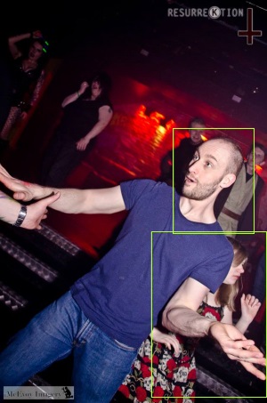
So, initially, I tried specifying 500 training images, which resulted in an SVM that actually did a pretty good job. The group photo shown before had all of the maybe-face regions correctly classified (the faces were all identified as faces and the hands in the photos were all correctly classified as not-faces).
However, there was a problem with the image shown here (the problem, btw, clearly isn't the moves being thrown on the dancefloor, since they look like the very essence of poetry in motion). The problem is that one of the maybe-face regions identified by the skin tone pass has been mis-classified by the SVM as a face, when it's really an arm.
(Note that there are some faces in the background that were not identified by the skin tone pass, but I'm not worried about that - it is to be expected that they would be ignored because they are small, relative to the size of the image.. though it should be possible to tweak the skin tone filter parameters if you wanted to try to capture background faces).
Increasing the number of training images to 1,000 didn't address the problem with this particular image and, in fact, made another image worse (where a non-face region was correctly classified as not-a-face before, with 1,000 training images the SVM thought that it was a face). Increasing to 1,500 training images corrected the classification of the dancing image regions but there were still false positives in other images. Such as this one of that same individual who appears to now be wearing a flag (which reminds me of a scene from Fear and Loathing in Las Vegas).
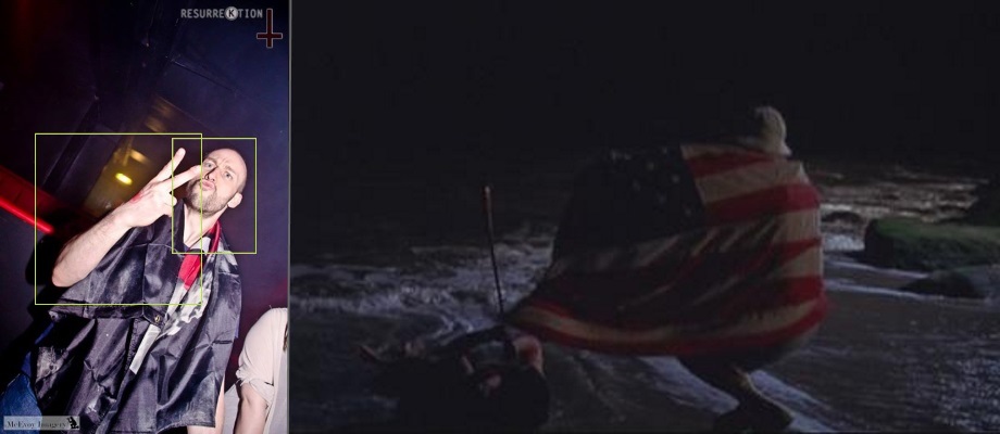
2,000 training images seemed to be the sweet spot. The classifier produced the correct results for every case that I expected it to.
The quantity of training data is going to vary from application to application and will depend upon what sort of feature extraction logic you are using. I think that it makes sense to start with lower quantities, if only because it's faster to train an SVM with less data and you can experiment more quickly with the other variables. To illustrate, on my computer (with the code as it currently stands, which is in a completely unoptimised state, but running a release build) it takes 17s to load the 2,000 images and extract the features from them, it then takes 27s to train the SVM on them. With 500 images it takes 5s to load the image data and 2s to train the SVM. With 5,000 images it takes 42s and 168s.

There's one final tweak that I'd like to mention before bringing everything to a close. The SVM requires that the inputs be fixed dimensions, so the "IsFace" implementation resizes the input image if it's too big or too small. If it's the wrong dimensions, though, then it leaves black bars above-and-below or left-and-right of the input (which is part of the process that I described in "Feature extraction for maybe-a-face images"). I found that the classification accuracy improved slightly if I expanded the maybe-a-face region so that it matched the aspect ratio of the SVM's input dimensions first. For example, if the skin tone pass identified a face region that was 91x241px and I knew that the SVM was configured to work with input images of 128x128px then I would first expand the 91x241px region to 241x241px (similarly, if I had a region that was 123x56px then I would expand it to 123x123px).
Performance
In the context of this kind of work, "performance" relates to two distinct areas - how accurately does it perform its work and how quickly does it do it? To an extent, the two are related since we could make the skin tone filter work more quickly (if we reduced the limit from no-input-dimension-may-be-more-than-400px to 300px or 200px) but at the risk of it no longer identifying regions that we want it to. As we've just seen with the SVM training, the time it takes to train it depends upon the quantity of data (both the size of the input image that features are extracted from and the number of input images) - so the inputs could be reduced (so that the training time would be shorter) but this negatively affects the accuracy of the classifier.
(A handy tip that I used when I was happy with the SVM training but experimenting with the skin tone pass was that the Accord.NET SVM class may be serialised using the BinaryFormatter - so I was persisting it to disk between runs, rather than having to re-train it on every run)
Once the SVM is trained, it is very quick at classifying. Which makes sense, since all it needs to do is take a feature set, apply its linear formula and see which side of the hyperplane the data point sits on. There is a little work required to extract the feature data from a maybe-face sub-image in order to give the SVM something to work on but it takes less then 15ms per sub-image on my computer. The skin tone pass is slower, taking between 150 and 300ms for the images that I've been testing with (which are all about 1000px on the largest side and so are resized down to 400px before being processed). I'd like to cut this time down because I like the idea of being able to apply this processing to video and I feel that it needs to be able to process at least five frames a second to convincingly track faces. I haven't made any effort towards this yet but reducing the total time down to 200ms feels reasonable since the code has been written to be easy to follow and tweak, rather than to be fast, so there is surely plenty of performance tuning potential.
Another reason that I haven't spent any time optimising the current code is that it might be wiser to spend time researching alternative algorithms. For example, Accord.NET has some support for face detection, such as the FaceHaarCascade class (which I believe is the same class of detector as the Viola–Jones object detection framework) -
Rectangle[] faceRegions;
using (var image = new Bitmap(path))
{
    var detector = new HaarObjectDetector(new FaceHaarCascade());
    faceRegions = detector.ProcessFrame(image);
}
However, it gave poor results for my images. It seemed to do well with very small faces but struggled with larger images (or the images where the faces took up a large proportion of the image). It's very possible that I could improve the accuracy by tweaking the parameters. If my images are too large, maybe they should just be shrunk down further before processing? That might help the false negative rate but I'm also concerned about the false positive rate and I'm not sure that shrinking the image first would help with that.
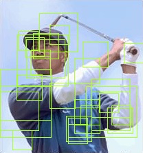
One approach that sounds very promising: if the SVM classifier is so fast and effective then maybe we should get rid of the skin tone processing altogether and just generate segments from all over the image, then filter them with the classifier. This is discussed and recommended by many people and is referred to as the "sliding window" approach (see Sliding Windows for Object Detection with Python and OpenCV, for example). The idea is that you pick a window size (eg. 50px if limiting the source image to no more than 400px on a side) and then start at the top left of the image and take that top-left 50x50px as the first sub-image to pass to the classifier. Then you move the window over a bit (say, 10px) and then use that as the second sub-image. Keep going until you can't go any further and then go back to the left but go down 10px - moving across then back-and-down until you have covered the entire image. Then do the same with some other window sizes (maybe 75px and then 100px), since you don't know whether the faces on an image are going to be small (relative to the size of the image) or large. This will give you many, many regions to classify - but that's no problem because linear SVM classification is very fast. Unfortunately, I did try this but I got an enormous false positive rate (as you can see here with Tiger - if you can make him out from behind all the green "this is a face!" boxes). Surely this approach can be made to work since it's so commonly presented as a solution to this problem.. it may just be that I need to tweak how the SVM is trained, maybe it needs more than 2,000 training images (though I did also try it with 10,000 training images and the results were not much better).

To return to the performance of the skin-tone-pass-following-by-(2k-image-trained-)SVM-classification model that I've talked about for most of this post; in terms of accuracy I'm very happy with it. In the test images that I've been using, there are zero false positives. There are a couple of false negatives but I think that they are understandable. The first obvious failing that it has is with a black-and-white photo - since the skin tone face detector looks for particular hues and saturations, it's not going to work on if there is no colour in the image. That's just a built-in limitation of the approach.
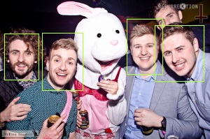
Another failure is with a face that is half hidden behind someone else (in the top right of this group photo). The skin tone face detector identifies the face but the SVM classifies it as not-a-face. Since the face is half-hidden, I think that this is acceptable.
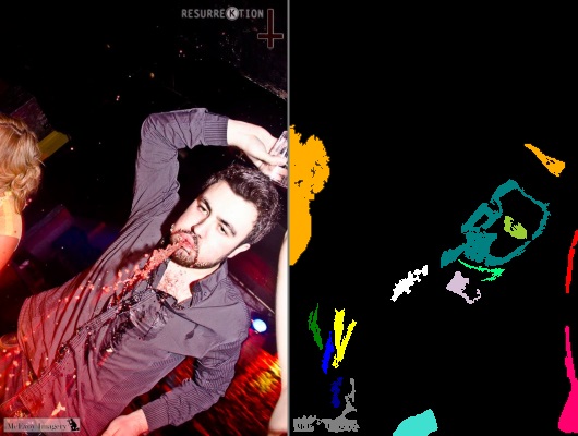

Last but not least is this unfortunate guy who foolishly entered some sort of drinking contest. I don't know if he won but he doesn't look too good about it one way or the other. The red liquid erupting from his lips falls within the first phase's looks-like-skin-tones bounds, as you can see by looking at the skin mask image. Not only is his head tilted in the shot but the vomit-detected-as-skin means that his face isn't centered in the maybe-face region. So I'm not surprised that the SVM doesn't correctly classify it.
In summary, it's not perfect but I'm still very happy with the results.
Article references
I want to close this post off by linking to the sites and papers that helped me get to this point. It's been a fun journey and is hopefully only my first step on the machine learning track!
The "Naked People Skin Filter (Fleck & Forsyth)" and "Face Detection in Color Images" papers were amongst the first that I found that had easily understandable material (for a face detection novice) that didn't use a third party library in some way.
Once I had implemented the skin tone logic and was looking to improve the results, one of the articles that I found most inspiring (partly because it was so approachable) was "Machine Learning is Fun! Part 4: Modern Face Recognition with Deep Learning" (by Adam Geitgey). This talks about taking things to the next step and performing facial recognition - not just locating faces but also trying to identify who they are, against a known database. I haven't got to that advanced point yet but it's definitely something that I'd like to explore. The only thing that I would say about this article is that it doesn't go into a lot of depth about generating HOGs or normalising them or what sort of input image size and other parameters to use. He does link to some Python code that uses third party libraries in lieu of more details, though. Since I wanted to write C# and (ideally) only take C# dependencies this wasn't very helpful to me. The article itself, though, got me really excited about the possibilities and I enjoyed the guy's writing style (and intend to read the rest of his "Machine Learning is Fun" series).
An article that did go into the details was the "HOG Person Detector Tutorial" (by Chris McCormick). This was also really well written and very approachable. Although it talks about detecting a person in a photo, rather than a face, the principles are the same. The description of the HOG generation and normalisation really helped me clarify in my mind how it should all work. This article links to the original HOG person detector paper by Dalal and Triggs [PDF], which is full of research information and graphs and equations - so if you want to dig deep then this is the place to start!
The Triggs and Dalal paper state in the introduction that "For simplicity and speed, we use linear SVM as a baseline classifier throughout the study". Later on they mention that they tried a non-linear kernel but that "Replacing the linear SVM with a Gaussian kernel one improves performance by about 3%.. at the cost of much higher run times". If this "why is a linear SVM classifier appropriate" explanation feels too light for you then it is discussed in greater depth in "Why do linear SVMs trained on HOG features perform so well? [PDF].
Finally, I want to mention again the article "Kernel Support Vector Machines for Classification and Regression in C#" by Accord.NET's César Souza. Here, he introduces the SVM in a much more formal way than I've done here, he includes a video about "The Kernel Trick" (which is a simple yet mind-blowing way in which the linear kernel can be used to classify data that doesn't immediately look like it would work for), he talks about other kernels (aside from linear he also describes polynomial and gaussian) and he describes how the Sequential Minimal Optimization learning algorithm works. There's a lot of code and there's illustrated examples at the end. When I found this article fairly early on in my research, I recognised how much care had gone into preparing it but also knew that I needed something a little more beginner-level first! So I bookmarked it for future reference and now I think that I understand (almost all of) it. Hopefully, if you started off knowing nothing but have followed all the way through this post, then you will too!
Posted at 18:39
About
Dan is a big geek who likes making stuff with computers! He can be quite outspoken so clearly needs a blog :)
In the last few minutes he seems to have taken to referring to himself in the third person. He's quite enjoying it.
Recent Posts
- Hosting a DigitalOcean App Platform app on a custom subdomain (with CORS)
- (Approximately) correcting perspective with C# (fixing a blurry presentation video - part two)
- Finding the brightest area in an image with C# (fixing a blurry presentation video - part one)
- So.. what is machine learning? (#NoCodeIntro)
- Parallelising (LINQ) work in C#
Highlights
- Face or no face (finding faces in photos using C# and Accord.NET)
- When a disk cache performs better than an in-memory cache (befriending the .NET GC)
- Performance tuning a Bridge.NET / React app
- Creating a C# ("Roslyn") Analyser - For beginners by a beginner
- Translating VBScript into C#
- Entity Framework projections to Immutable Types (IEnumerable vs IQueryable)
Archives
- April 2025 (1)
- March 2022 (2)
- February 2022 (1)
- August 2021 (1)
- April 2021 (2)
- March 2021 (1)
- August 2020 (3)
- July 2019 (2)
- September 2018 (1)
- April 2018 (1)
- March 2018 (1)
- July 2017 (1)
- June 2017 (1)
- February 2017 (1)
- November 2016 (1)
- September 2016 (2)
- August 2016 (1)
- July 2016 (1)
- June 2016 (1)
- May 2016 (3)
- March 2016 (3)
- February 2016 (2)
- December 2015 (1)
- November 2015 (2)
- August 2015 (3)
- July 2015 (1)
- June 2015 (1)
- May 2015 (2)
- April 2015 (1)
- March 2015 (1)
- January 2015 (2)
- December 2014 (1)
- November 2014 (1)
- October 2014 (2)
- September 2014 (2)
- August 2014 (1)
- July 2014 (1)
- June 2014 (1)
- May 2014 (2)
- February 2014 (1)
- January 2014 (1)
- December 2013 (1)
- November 2013 (1)
- October 2013 (1)
- August 2013 (3)
- July 2013 (3)
- June 2013 (1)
- May 2013 (2)
- April 2013 (1)
- March 2013 (8)
- February 2013 (2)
- January 2013 (2)
- December 2012 (3)
- November 2012 (4)
- September 2012 (1)
- August 2012 (1)
- July 2012 (3)
- June 2012 (3)
- May 2012 (2)
- February 2012 (3)
- January 2012 (4)
- December 2011 (7)
- August 2011 (2)
- July 2011 (1)
- May 2011 (1)
- April 2011 (2)
- March 2011 (3)